ImageNet Classification with Deep Convolutional Neural Networks
1. Introduction
Convolutional neural networks (CNNs) constitute one such class of models [16, 11, 13, 18, 15, 22, 26]. Their capacity can be controlled by varying their depth and breadth, and they also make strong and mostly correct assumptions about the nature of images (namely, stationarity of statistics and locality of pixel dependencies). Thus, compared to standard feedforward neural networks with similarly-sized layers, CNNs have much fewer connections and parameters and so they are easier to train, while their theoretically-best performance is likely to be only slightly worse.
- Stationarity of Statistics: Images’ statistical properties, such as texture and color distributions, are assumed to be consistent across different regions of the image. This enables CNNs to apply the same filters to the entire image, significantly reducing the model’s complexity.
- Locality of Pixel Dependencies: CNNs operate under the assumption that nearby pixels are more likely to be connected. In order to enable the network to recognize local features like edges and shapes, this is accomplished by applying tiny, localized filters (kernels) to the image.
Mathematically, a convolution operation in a CNN can be represented as:
\[f(x, y) = \sum_{i=-a}^{a} \sum_{j=-b}^{b} K(i, j) \cdot I(x-i, y-j)\]Here, ( f(x, y) ) is the output after applying the convolution operation to the input image ( I ) at position ( (x, y) ). The kernel ( K(i, j) ) is applied over the image such that each element of the kernel is multiplied by the corresponding element of the image under it, and the results are summed to produce the output ( f(x, y) ). The kernel ( K ) can be expressed as a matrix:
\[K = \begin{bmatrix} k_{11} & k_{12} & k_{13} \\ k_{21} & k_{22} & k_{23} \\ k_{31} & k_{32} & k_{33} \end{bmatrix}\]With fewer parameters than fully connected networks, CNNs can learn hierarchical representations of images thanks to these principles, which makes them particularly useful for tasks like object detection and image classification.
2. Dataset
ImageNet is a dataset of over 15 million labeled high-resolution images belonging to roughly 22,000 categories.
3. The Architecture
3.1 ReLU Nonlinearity
In terms of training time with gradient descent, these saturating nonlinearities are much slower than the non-saturating nonlinearity f(x) = max(0,x). Following Nair and Hinton [20], we refer to neurons with this nonlinearity as Rectified Linear Units (ReLUs). Deep convolutional neural net- works with ReLUs train several times faster than their equivalents with tanh units.
The activation function is a core component in neural networks that introduces non-linearity, affecting the network’s ability to learn complex patterns. Traditional activation functions like the hyperbolic tangent (tanh) or the sigmoid function can cause the gradient to vanish during backpropagation, which slows down the training.
The Rectified Linear Unit (ReLU) has become the de facto standard in neural network activation due to its non-saturating form, defined as:
\[ReLU(x) = \max(0, x)\]This simple yet powerful function maintains the gradient, preventing the vanishing gradient problem and allowing the network to learn faster. Neurons with ReLU activation are only activated when the input is positive, leading to sparse activation within the network.
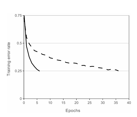
CNNs with ReLUs train substantially faster than those with tanh units. This efficiency gain is depicted in the figure below, which demonstrates how a four-layer convolutional network with ReLUs can reach a 25% training error rate on CIFAR-10 much quicker than the same network utilizing tanh neurons.

Empirical results show that networks with ReLU not only train faster but also achieve better performance on complex tasks, which is particularly beneficial when dealing with large datasets and deep architectures.
3.3 Local Response Normalization
ReLUs have the desirable property that they do not require input normalization to prevent them from saturating. If at least some training examples produce a positive input to a ReLU, learning will happen in that neuron. However, we still find that the following local normalization scheme aids generalization.
The Role in ReLU Networks
While Rectified Linear Units (ReLUs) have the advantage of not requiring input normalization to prevent saturation, we discovered an additional normalization technique that enhances generalization. This is known as Local Response Normalization (LRN).
Mechanism of LRN
Given the activity \(a*{i}^{x,y}\) of a neuron, calculated by applying \(kernel ( i )\) at position \((x, y)\) and then passing it through a ReLU nonlinearity, the response-normalized activity \(( b*{i}^{x,y} )\) can be described by:
\[b_{i}^{x,y} = \frac{a_{i}^{x,y}}{\left(k + \alpha \sum_{j=\max(0, i-n/2)}^{\min(N-1, i+n/2)} (a_{j}^{x,y})^2\right)^\beta}\]Here, the sum runs over ( n ) “adjacent” kernel maps at the same spatial position, and ( N ) represents the total number of kernels in the layer. This normalization is inspired by lateral inhibition found in biological neurons, inducing competition among neuron outputs computed with different kernels.
3.4 Overlapping Pooling
If a pooling layer has a grid of pooling units, they are spaced s pixels apart and each summarizes a z × z neighborhood. Traditional pooling sets s = z, meaning no overlap between the neighborhoods.
However, Imagenet employs an overlapping pooling strategy. They set s < z. Specifically, we use s = 2 and z = 3. This overlapping approach has been found to be more effective in reducing error rates.
3.5 Overall Architecture
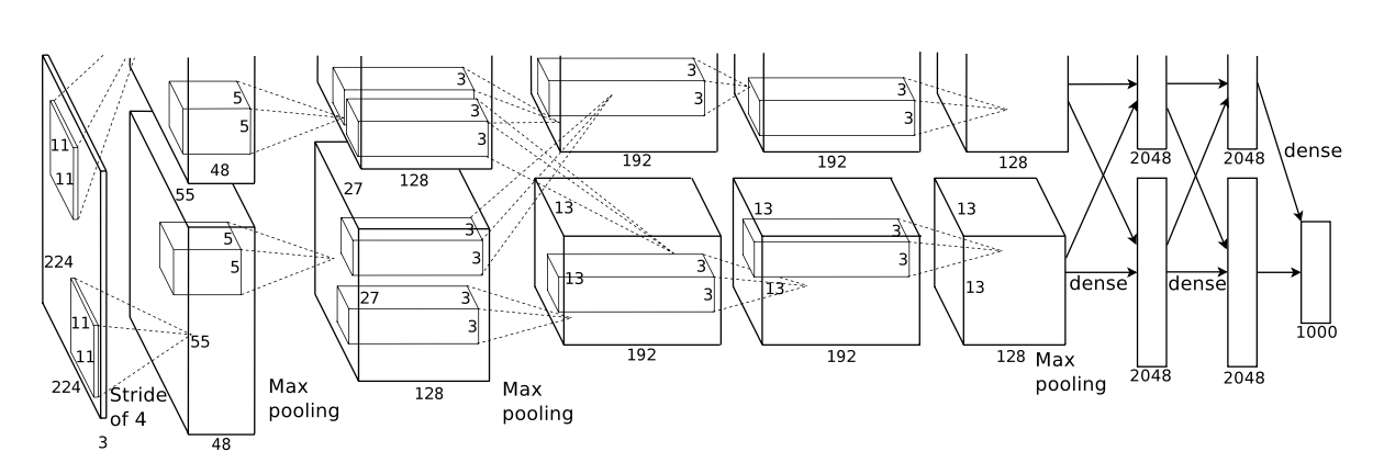
As depicted in Figure 2, the net contains eight layers with weights; the first five are convolutional and the remaining three are fully- connected. The output of the last fully-connected layer is fed to a 1000-way softmax which produces a distribution over the 1000 class labels. Our network maximizes the multinomial logistic regression objective, which is equivalent to maximizing the average across training cases of the log-probability of the correct label under the prediction distribution.
The approximately 60 million trainable parameters of Imagenet are a crucial component. This large number of parameters improves the network’s classification performance by enabling it to learn intricate and subtle features from the vast and diverse ImageNet dataset. Throughout the training phase, these parameters are changed to allow the network to perform as well as possible on the dataset.

Imagenet(
  (features): Sequential(
    (0): Conv2d(3, 64, kernel_size=(11, 11), stride=(4, 4), padding=(2, 2)) // 23,232 parameters
    (1): ReLU(inplace=True)
    (2): MaxPool2d(kernel_size=3, stride=2, padding=0, dilation=1, ceil_mode=False)
    (3): Conv2d(64, 192, kernel_size=(5, 5), stride=(1, 1), padding=(2, 2)) // 307,200 parameters
    (4): ReLU(inplace=True)
    (5): MaxPool2d(kernel_size=3, stride=2, padding=0, dilation=1, ceil_mode=False)
    (6): Conv2d(192, 384, kernel_size=(3, 3), stride=(1, 1), padding=(1, 1)) // 663,552 parameters
    (7): ReLU(inplace=True)
    (8): Conv2d(384, 256, kernel_size=(3, 3), stride=(1, 1), padding=(1, 1)) // 884,736 parameters
    (9): ReLU(inplace=True)
    (10): Conv2d(256, 256, kernel_size=(3, 3), stride=(1, 1), padding=(1, 1)) // 589,824 parameters
    (11): ReLU(inplace=True)
    (12): MaxPool2d(kernel_size=3, stride=2, padding=0, dilation=1, ceil_mode=False)
  )
  (avgpool): AdaptiveAvgPool2d(output_size=(6, 6))
  (classifier): Sequential(
    (0): Dropout(p=0.5, inplace=False)
    (1): Linear(in_features=9216, out_features=4096, bias=True) // 37,748,736 parameters
    (2): ReLU(inplace=True)
    (3): Dropout(p=0.5, inplace=False)
    (4): Linear(in_features=4096, out_features=4096, bias=True) // 16,777,216 parameters
    (5): ReLU(inplace=True)
    (6): Linear(in_features=4096, out_features=1000, bias=True) // 4,096,000 parameters
  )
)
4 Reducing Overfitting
Our neural network architecture has 60 million parameters. Although the 1000 classes of ILSVRC make each training example impose 10 bits of constraint on the mapping from image to label, this turns out to be insufficient to learn so many parameters without considerable overfitting. Below, we describe the two primary ways in which we combat overfitting.
4.1 Data Augmentation
We employ two distinct forms of data augmentation
- Generating image translations and horizontal reflections
- PCA Color Augmentation
PCA Color Augmentation
PCA Color Augmentation is a technique to augment image data by adjusting the intensities of the RGB channels. This method helps the model become more invariant to changes in illumination, which is a common property of natural images.
The process involves the following steps:
- Perform PCA on the RGB pixel values across the entire ImageNet training set to obtain principal components.
- For each training image, alter the pixel values by adding a certain amount of these principal components.
Mathematically, for each pixel \(I\_{xy} = [I_R, I_G, I_B]^T\) in the image, we add the following quantity:
\[[p_1, p_2, p_3][\alpha_1 \lambda_1, \alpha_2 \lambda_2, \alpha_3 \lambda_3]^T\]Here:
- \(p_i\) represents the \(i\)-th eigenvector from the PCA of the RGB pixel values.
- \(\lambda_i\) is the corresponding eigenvalue, which indicates the variance in the direction of the eigenvector.
- \(\alpha_i\) is a random variable drawn from a Gaussian distribution with mean zero and standard deviation 0.1. It is sampled once per image and used across all pixels, ensuring consistency within the image.
By scaling the principal components by their corresponding eigenvalues and the random variable, we effectively simulate realistic variations in lighting. This adjustment to the pixel values does not alter the content or structure of the image, preserving the label of the image while providing a form of regularization.
4.2 Dropout
The recently-introduced technique, called “dropout” [10], consists of setting to zero the output of each hidden neuron with probability 0.5. The neurons which are “dropped out” in this way do not contribute to the forward pass and do not participate in back- propagation. So every time an input is presented, the neural network samples a different architecture, but all these architectures share weights. This technique reduces complex co-adaptations of neurons, since a neuron cannot rely on the presence of particular other neurons. It is, therefore, forced to learn more robust features that are useful in conjunction with many different random subsets of the other neurons.
To stop overfitting in neural networks, dropout is a regularization technique used. The network is forced to learn robust features that are independent of any particular set of neurons by randomly setting a portion of the neuron outputs to zero during training. Overfitting is essentially reduced by the randomness in neuron activation, which improves the model’s ability to generalize to new data. Neuron outputs are adjusted to compensate for the deactivated neurons during training, but dropout is not applied during testing.
Results
Comparison of Model Performances
The paper presents a comparison of the convolutional neural network (CNN) model with other notable methods. Below is a summary of their performances on the ImageNet Large Scale Visual Recognition Challenge (ILSVRC) for the years 2010 and 2012:
| Model | Top-1 Error (ILSVRC-2010) | Top-5 Error (ILSVRC-2010) | Top-5 Error (ILSVRC-2012) |
|---|---|---|---|
| CNN | 37.5% | 17.0% | 15.3% |
| Sparse Coding [2] | 47.1% | 28.2% | 26.2% (val) |
| SIFT + FVs [24] | 45.7% | 25.7% | - |
Analysis
- CNN: Demonstrates a notable decrease in the top-1 and top-5 error rates. This demonstrates how deep convolutional neural networks work well for tasks involving image classification.
- Sparse Coding [2]: Even though it works well, this approach has higher error rates than CNN, which highlights how much better deep learning techniques perform.
- SIFT + FVs [24]: It shows higher error rates, just like Sparse Coding. The comparison demonstrates how CNNs have improved at handling challenging image recognition tasks.
This comparative analysis illustrates the groundbreaking impact of CNNs in reducing error rates and setting new benchmarks in image classification.
Conclusion
By utilizing the expansive ImageNet dataset, the network achieved remarkable accuracy, showcasing a significant leap over previous state-of-the-art results. Key innovations include the use of ReLU nonlinearity, dropout for overfitting reduction, and extensive data augmentation, contributing to the network’s robust performance.
Citation
Krizhevsky, A., Sutskever, I., & Hinton, G. E. (2012). ImageNet Classification with Deep Convolutional Neural Networks. NIPS.