FlowNet Learning Optical Flow with Convolutional Networks

Exploring the Innovations in Flownet paper approach for optical flow estimation.

Abstract

Convolutional neural networks (CNNs) have recently been very successful in a variety of computer vision tasks, especially on those linked to recognition. Optical flow estimation has not been among the tasks CNNs succeeded at. In this paper we construct CNNs which are capable of solving the optical flow estimation problem as a supervised learning task. We propose and compare two architectures: a generic architecture and another one including a layer that correlates feature vectors at different image locations. Since existing ground truth data sets are not sufficiently large to train a CNN, we generate a large synthetic Flying Chairs dataset. We show that networks trained on this unrealistic data still generalize very well to existing datasets such as Sintel and KITTI, achieving competitive accuracy at frame rates of 5 to 10 fps.

Introduction

optical flow estimation needs precise per-pixel localization, it also requires finding correspondences between two input images. This involves not only learning image feature representations, but also learning to match them at different locations in the two images. In this respect, optical flow estimation fundamentally differs from previous applications of CNNs.

Figure 1:Efficacy of Correlation Layer in CNNs for Optical Flow Prediction.

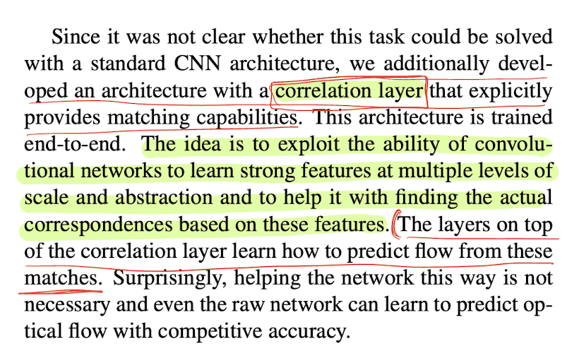
The network intorduces a new layer called correlation layer that significantly improves optical flow estimation by efficiently finding correspondences between different image patches.

Network Architectures

This paper takes an end-to-end learning approach to predicting optical flow: given a dataset consisting of image pairs and ground truth flows, we train a network to predict the x–y flow fields directly from the images.

Pooling in CNNs is necessary to make network training computationally feasible and, more fundamentally, to allow aggregation of information over large areas of the input images

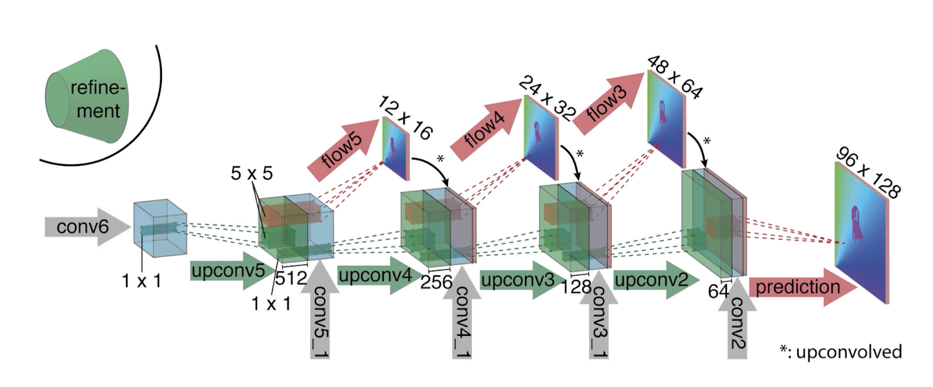
Networks consisting of contracting and expanding parts are trained as a whole using backpropagation. Architectures we use are depicted in Figures 3 and 4.

Contracting part

• A simple choice is to stack both input images together and feed them through a rather generic network, allowing the network to decide itself how to process Figure 2. Refinement of the coarse feature maps to the high resothe image pair to extract the motion information. This is illution prediction. lustrated in Figure 3.

• Another approach is to create two separate, yet identical processing streams for the two images and to combine them at a later stage as shown in Fig. 3. With this architecture the network is constrained to first produce meaningful representations of the two images separately and then combine them on a higher level

Correlation Layer in FlowNet

The correlation layer is a pivotal component of FlowNet’s architecture, allowing the network to compare patches from feature maps \(( f_1 )\) and \(( f_2 )\) derived from two input images. This comparison is fundamental for optical flow estimation, as it involves finding correspondences between different locations in these images.

Mathematical Formulation

The correlation of two patches centered at \(( x_1 )\)in the first map and \(( x_2 )\) in the second map is defined as:

\[c(x_1, x_2) = \sum_{o \in [-k, k] \times [-k, k]} \langle f_1(x_1 + o), f_2(x_2 + o) \rangle\]

where \(( \langle \cdot, \cdot \rangle )\) denotes the scalar product, and the summation is over a square patch of size \(( K := 2k + 1 )\). This equation is similar to a convolution operation but involves convolving data with other data, not with a filter.

Computational Considerations

For each location \(( x_1 )\), the correlations \(( c(x_1, x_2) )\) are computed only in a neighborhood of size \(( D := 2d + 1 )\), where \(( d )\) is the maximum displacement allowed. This is to make the computation tractable, as comparing all possible patch combinations without this limitation would be computationally expensive.

The computational cost of computing \(( c(x_1, x_2) )\) involves \(( c \cdot K^2 )\) multiplications, and the total cost for all patch combinations is proportional to \(( w^2 \cdot h^2 )\), where \(( w )\) and \(( h )\) are the width and height of the feature maps.

Implementation

In practice, the output of the correlation layer is organized into channels, representing relative displacements. This results in an output size of \(( (w \times h \times D^2) )\). For the backward pass, derivatives are implemented with respect to each input feature map.

estimates the computational complexity for computing feature map correlations, factoring in patch size (K), dimensions (w and h), and channel count (c) of the feature maps.

Figure 2: Flownet simple.

If we notice the architecture we see that the images are stacked together channel wise.

Figure 3: Flownet Corelation.

Expanding part

The main ingredient of the expanding part are upconvolutional layers, consisting of unpooling (extending the feature maps, as opposed to pooling) and a convolution. Such layers have been used previously [38, 37, 16, 28, 9]. To perform the refinement, we apply the ‘upconvolution’ to feature maps, and concatenate it with corresponding feature maps from the ’contractive’ part of the network and an upsampled coarser flow prediction (if available). This way we preserve both the high-level information passed from coarser feature maps and fine local information provided in lower layer feature maps. Each step increases the resolution twice. We repeat this 4 times, resulting in a predicted flow for which the resolution is still 4 times smaller than the input.

Figure 4: refinement-layrer.

Datasets

Flying Chairs The Sintel dataset is still too small to train large CNNs. To provide enough training data, we create a simple syn- thetic dataset, which we name Flying Chairs, by applying affine transformations to images collected from Flickr and a publicly available set of renderings of 3D chair models [1]. We retrieve 964 images from Flickr2 with a resolution of 1, 024 × 768 from the categories ‘city’ (321), ‘landscape’ (129) and ‘mountain’ (514). We cut the images into 4 quad- rants and use the resulting 512 × 384 image crops as back- ground. As foreground objects we add images of multi- ple chairs from [1] to the background. From the original dataset we remove very similar chairs, resulting in 809 chair types and 62 views per chair available. Examples are shown in Figure 5. To generate motion, we randomly sample 2D affine transformation parameters for the background and the chairs. The chairs’ transformations are relative to the back- ground transformation, which can be interpreted as both the camera and the objects moving. Using the transformation parameters we generate the second image, the ground truth optical flow and occlusion regions.

Results

Method	Sintel Clean train	Sintel Clean test	Sintel Final train	Sintel Final test	KITTI train	KITTI test	Middlebury train	Middlebury test	Chairs test	Time (sec) CPU	Time (sec) GPU
EpicFlow [30]	2.27	4.12	3.57	6.29	3.47	3.8	0.31	3.55	2.94	16	-
DeepFlow [35]	3.19	5.38	4.40	7.21	4.58	5.8	0.21	4.22	3.53	17	-
EPPM [3]	-	6.49	-	8.38	-	9.2	-	3.36	-	-	0.2
LDOF [6]	4.19	7.56	6.28	9.12	13.73	12.4	0.45	4.55	3.47	65	2.5
FlowNetS	4.50	7.42	5.45	8.43	8.26	-	1.09	-	2.71	-	0.08
FlowNetS+v	3.66	6.45	4.76	7.67	6.50	-	0.33	-	2.86	-	1.05
FlowNetS+ft	6.96	7.76	7.76	7.22	7.52	9.1	15.20	-	3.04	-	0.08
FlowNetS+ft+v	6.16	7.22	7.22	7.22	6.07	7.6	3.84	0.47	4.58	-	1.05
FlowNetC	4.31	7.28	5.87	8.81	9.35	-	15.64	-	2.19	-	0.15
FlowNetC+v	3.57	6.27	5.25	8.01	7.45	-	3.92	-	2.61	-	1.12
FlowNetC+ft	6.85	8.51	8.51	7.88	7.31	-	12.33	-	2.27	-	0.15
FlowNetC+ft+v	6.08	7.88	7.88	7.88	6.07	7.6	3.81	0.50	4.52	-	1.12

This Table represents Average endpoint errors (in pixels) of our networks compared to several well-performing methods on different datasets. The numbers in parentheses are the results of the networks on data they were trained on, and hence are not directly comparable to other results.

• FlowNetS generalizes better to datasets with additional complexities such as motion blur or fog, as evidenced by its performance on the Sintel Final dataset. In contrast, FlowNetC performs better on datasets with fewer complexities, such as Flying Chairs and Sintel Clean, indicating a proclivity to overfit to the type of data encountered during training. Despite having similar numbers of parameters, FlowNetC's overfitting may be advantageous with better training data.

• Furthermore, FlowNetC appears to struggle more with large displacements than FlowNetS, as demonstrated by its performance on the KITTI dataset and detailed analysis on Sintel Final. The constraint on maximum displacement within FlowNetC's correlation layer may be the limiting factor, which can be adjusted at the expense of computational efficiency.

Conclusion

Building on recent progress in design of convolutional network architectures, we have shown that it is possible to train a network to directly predict optical flow from two in- put images. Intriguingly, the training data need not be re- alistic. The artificial Flying Chairs dataset including just affine motions of synthetic rigid objects is sufficient to pre- dict optical flow in natural scenes with competitive accu- racy. This proves the generalization capabilities of the pre- sented networks. On the test set of the Flying Chairs the CNNs even outperform state-of-the-art methods like Deep- Flow and EpicFlow. It will be interesting to see how future networks perform as more realistic training data becomes available.

---