GPU Optimization for Convolution Operations
A comprehensive analysis of convolution operations on GPUs, focusing on theoretical foundations, performance metrics, and optimization strategies.
1. Introduction
In this blog we are gonna explore the convolution operation, and how accleration of this operation uisng the Nvidia-cuda toolkit and various perfoamce measure and metrics along the way.
2. Theoretical Foundations of Convolution Operations
2.1 Mathematical Definition
For an input tensor $\mathcal{I}$ and a filter tensor $\mathcal{F}$, the 2D convolution operation can be expressed as:
\[\mathcal{O}_{n,k,i,j} = \sum_{c=0}^{C_{in}-1} \sum_{p=0}^{K_h-1} \sum_{q=0}^{K_w-1} \mathcal{I}_{n,c,i+p,j+q} \cdot \mathcal{F}_{k,c,p,q}\]Where:
- $\mathcal{O}$ is the output tensor
- $n$ is the batch index
- $k$ is the output channel index
- $i, j$ are spatial indices in the output
- $c$ is the input channel index
- $p, q$ are spatial indices in the filter
- $C_{in}$ is the number of input channels
- $K_h, K_w$ are the height and width of the filter
2.2 Tensor Dimensions
Given:
- Input tensor $\mathcal{I} \in \mathbb{R}^{N imes C_{in} imes H_{in} imes W_{in}}$
- Filter tensor $\mathcal{F} \in \mathbb{R}^{C_{out} imes C_{in} imes K_h imes K_w}$
The output tensor $\mathcal{O}$ will have dimensions:
\[\mathcal{O} \in \mathbb{R}^{N imes C_{out} imes H_{out} imes W_{out}}\]Where: \(H_{out} = H_{in} - K_h + 1\) \(W_{out} = W_{in} - K_w + 1\)
2.3 Visual Representation of Convolution Operation
Example Configuration
- Input Tensor:
N=1, C=4, H=4, W=4 - Filter Tensor:
N=1, C=4, H=2, W=2 - Output Tensor: The output tensor dimensions are calculated as follows:
Output Dimensions Calculation
The output dimensions are computed as:
\(H_{out} = H_{in} - K_h + 1 = 4 - 2 + 1 = 3\) \(W_{out} = W_{in} - K_w + 1 = 4 - 2 + 1 = 3\)
Therefore, the output tensor has dimensions N=1, C=1, H=3, W=3.
2.3.1 Visualizing the 3D Convolution Operation
Input Tensor (H=4, W=4, C=4)
Each layer represents one of the 4 channels of the input tensor.
Channel 1                Channel 2                Channel 3                Channel 4
-------------------      -------------------      -------------------      -------------------
| 1 | 2 | 0 | 1 |        | 1 | 0 | 1 | 2 |        | 0 | 1 | 2 | 1 |        | 1 | 2 | 1 | 0 |
| 0 | 1 | 3 | 2 |        | 2 | 1 | 0 | 1 |        | 1 | 2 | 0 | 1 |        | 2 | 0 | 1 | 1 |
| 1 | 2 | 1 | 0 |        | 0 | 1 | 2 | 0 |        | 1 | 1 | 0 | 2 |        | 0 | 1 | 2 | 2 |
| 2 | 1 | 0 | 1 |        | 2 | 0 | 1 | 1 |        | 2 | 0 | 1 | 0 |        | 1 | 0 | 1 | 1 |
-------------------      -------------------      -------------------      -------------------
Filter Tensor (H=2, W=2, C=4)
Each layer represents one of the 4 channels of the filter tensor.
Channel 1                Channel 2                Channel 3                Channel 4
-------------------      -------------------      -------------------      -------------------
| 1 | 0 |                | 0 | 1 |                | 1 | 0 |                | 0 | 1 |
| 0 | 1 |                | 1 | 0 |                | 0 | 1 |                | 1 | 0 |
-------------------      -------------------      -------------------      -------------------
Convolution Operation Visualization (3D)
The convolution operation involves performing a dot product of the 4-channel filter tensor with the 4-channel input tensor over a 2x2 region.
3D Dot Product Representation
We loop over x---direction and one in y---direction input : [1,:,0:2,0:2] and slice the array get input: [1,:,:2,:2]* filter [1,:,:2,:2] This colapses channles and just returns the output
\(H_{out} = H_{in} - K_h + 1 = 4 - 2 + 1 = 3\) \(W_{out} = W_{in} - K_w + 1 = 4 - 2 + 1 = 3\)
3D Dot Product Operation for Each Spatial Position
+----------------------------+     +----------------------------+
| Input (4x2x2) Sub-Tensor   |     | Filter (4x2x2) Sub-Tensor  |
| for spatial position (0,0) |     |                          |
+----------------------------+     +----------------------------+
| [                         ] |     | [                         ] |
| Channel 1:                |     | Channel 1:                |
| [ 1 | 2 ]                 |     | [ 1 | 0 ]                 |
| [ 0 | 1 ]                 |     | [ 0 | 1 ]                 |
|                           |     |                           |
| Channel 2:                |     | Channel 2:                |
| [ 1 | 0 ]                 |     | [ 0 | 1 ]                 |
| [ 2 | 1 ]                 |     | [ 1 | 0 ]                 |
|                           |     |                           |
| Channel 3:                |     | Channel 3:                |
| [ 0 | 1 ]                 |     | [ 1 | 0 ]                 |
| [ 1 | 2 ]                 |     | [ 0 | 1 ]                 |
|                           |     |                           |
| Channel 4:                |     | Channel 4:                |
| [ 1 | 2 ]                 |     | [ 0 | 1 ]                 |
| [ 2 | 0 ]                 |     | [ 1 | 0 ]                 |
+----------------------------+     +----------------------------+
3D Convolution Result at Spatial Position (0,0)
Cumulative Sum for Output Tensor at (0,0):
1*1 + 2*0 + 0*1 + 1*0 + 1*0 + 0*1 + 2*1 + 1*0 + 0*1 + 1*0 + 1*1 + 2*0 + 1*0 + 2*1 + 0*0 + 2*0 = 8
This value is stored in the output tensor at position (0,0). We repeat this process for all spatial positions.
Final Output Tensor
Output Tensor (H=3, W=3, C=1):
-----------------
|  8 |  7 |  6 |
|  5 |  8 |  9 |
|  7 |  5 |  4 |
-----------------
Each value represents the cumulative dot product result for each corresponding spatial position in the input tensor.
This visualization demonstrates how the filter interacts with the input tensor across all channels to generate the output tensor values.
2.4 Padding and Stride
2.4.1 Padding
Padding is used to control the spatial size of the output tensor. With padding, zeros are added to the input tensor around its border to allow the filter to slide outside the input’s original spatial dimensions.
Example with Padding:
Input Tensor (5x5 with padding of 1):
-------------------------
| 0 | 0 | 0 | 0 | 0 | 0 | 0 |
| 0 | 1 | 2 | 0 | 1 | 2 | 0 |
| 0 | 0 | 1 | 3 | 2 | 1 | 0 |
| 0 | 1 | 2 | 1 | 0 | 1 | 0 |
| 0 | 2 | 1 | 0 | 1 | 0 | 0 |
| 0 | 1 | 2 | 0 | 1 | 2 | 0 |
| 0 | 0 | 0 | 0 | 0 | 0 | 0 |
-------------------------
2.4.2 Stride
Stride controls how the filter convolves around the input tensor. If the stride is 1, the filter moves one pixel at a time. If the stride is 2, it moves two pixels at a time.
Example with Stride 2:
Input Tensor:
-----------------
| 1 | 2 | 0 | 1 |
| 0 | 1 | 3 | 2 |
| 1 | 2 | 1 | 0 |
| 2 | 1 | 0 | 1 |
-----------------
Stride 2:
-----------------
| 1 | 0 |
| 1 | 1 |
-----------------
Output Tensor (2x2):
-----------------
|  7 |  6 |
|  6 |  3 |
-----------------
In this example, the filter skips every other position, resulting in a smaller output tensor.
2.4.3 Combining Padding and Stride
When using both padding and stride, we can control the exact size of the output tensor.
Example:
- Padding = 1, Stride = 2
- Input Tensor = 5x5 (with padding added)
- Output Tensor = 3x3
Input Tensor with Padding:
-------------------------
| 0 | 0 | 0 | 0 | 0 | 0 | 0 |
| 0 | 1 | 2 | 0 | 1 | 2 | 0 |
| 0 | 0 | 1 | 3 | 2 | 1 | 0 |
| 0 | 1 | 2 | 1 | 0 | 1 | 0 |
| 0 | 2 | 1 | 0 | 1 | 0 | 0 |
| 0 | 1 | 2 | 0 | 1 | 2 | 0 |
| 0 | 0 | 0 | 0 | 0 | 0 | 0 |
-------------------------

Output Tensor (3x3):
-----------------
|  4 |  5 |  2 |
|  3 |  6 |  1 |
|  5 |  3 |  3 |
-----------------
This explains how padding and stride can be used to control the size and shape of the output tensor, allowing for more flexibility in convolution operations.
2.5 Dilated Convolution
2.5.1 Introduction to Dilation
Dilated convolutions introduce “holes” in the filter, effectively increasing the receptive field without increasing the number of parameters or the amount of computation. This allows the model to capture more global information while maintaining the resolution.
2.5.2 Dilated Convolution Operation
In a dilated convolution, the filter is applied over an input tensor with defined gaps, controlled by the dilation rate. For example, a dilation rate of 2 means skipping one element between every two filter elements.
Example with Dilation 2:
Input Tensor:
-----------------
| 1 | 2 | 0 | 1 |
| 0 | 1 | 3 | 2 |
| 1 | 2 | 1 | 0 |
| 2 | 1 | 0 | 1 |
-----------------
Dilation 2:
-----------------
| 1 | 0 |
| 1 | 1 |
-----------------
Output Tensor (2x2):
-----------------
|  4 |  2 |
|  3 |  4 |
-----------------
2.5.3 Combining Dilation with Padding and Stride
Dilated convolutions can be combined with padding and stride to allow for more flexible receptive field adjustments.
Example:
- Padding = 1, Stride = 1, Dilation = 2
- Input Tensor = 5x5
- Output Tensor = 3x3
Input Tensor:
-----------------
| 1 | 2 | 3 | 4 | 5 |
| 6 | 7 | 8 | 9 | 0 |
| 1 | 2 | 3 | 4 | 5 |
| 6 | 7 | 8 | 9 | 0 |
| 1 | 2 | 3 | 4 | 5 |
-----------------
Filter:
-----------------
| 1 | 0 |
| 0 | 1 |
-----------------
Output Tensor (3x3):
-----------------
|  4 |  8 |  0 |
| 12 | 16 |  8 |
|  4 |  8 |  0 |
-----------------
This demonstrates how dilation, padding, and stride can be used together to control the receptive field, tensor size, and level of detail captured in the convolution operation.
3. Tensor Computations on GPUs
3.1 GPU Memory Hierarchy
GPUs have a complex memory hierarchy that affects the performance of tensor computations:
- Global Memory: Largest but slowest
- Capacity: Typically several GB
- Latency: 400-800 clock cycles
- Shared Memory: Fast, on-chip memory shared by threads in a block
- Capacity: Typically 48KB - 96KB per SM
- Latency: ~20 clock cycles
- Registers: Fastest, private to each thread
- Capacity: Typically 256KB per SM
- Latency: ~1 clock cycle
3.2 Tensor Operations in CUDA
In CUDA, tensor operations are typically implemented using multi-dimensional thread blocks. For a 4D tensor operation, we might use a 3D grid of thread blocks:
dim3 threadsPerBlock(BLOCK_SIZE_X, BLOCK_SIZE_Y, 1);
dim3 numBlocks(
    (W_out + BLOCK_SIZE_X - 1) / BLOCK_SIZE_X,
    (H_out + BLOCK_SIZE_Y - 1) / BLOCK_SIZE_Y,
    C_out
);
Each thread then computes one or more elements of the output tensor:
int w = blockIdx.x * blockDim.x + threadIdx.x;
int h = blockIdx.y * blockDim.y + threadIdx.y;
int c = blockIdx.z;
This mapping allows for efficient parallelization of tensor operations on GPUs.
In the next section, we will delve into NVIDIA performance metrics and how they relate to optimizing convolution operations.
3.3 Mapping Tensor Operations to CUDA
The given CUDA code performs a 2D convolution operation on an input tensor using the NCHW format, where:
-
Nrepresents the batch size. -
Crepresents the number of channels. -
HandWrepresent the height and width of the tensor, respectively.
3.3.1 Tensor Mapping to CUDA Thread Blocks
The input, filter, and output tensors are mapped to CUDA thread blocks and threads using 3D grid dimensions. Each thread computes a single element of the output tensor.
Input Tensor (NCHW)               Filter Tensor (OCHW)               Output Tensor (NCHW)
-----------------------           -----------------------            -----------------------
N = 1                             O = 2                              N = 1
C = 2                             C = 2                              C = 2
H = 5                             H = 3                              H = 3
W = 5                             W = 3                              W = 3

Input (1, 2, 5, 5)                Filter (2, 2, 3, 3)                Output (1, 2, 3, 3)


[ x x x x x ]                     [ w w w ]                          [ y y y ]
[ x x x x x ]                     [ w w w ]                          [ y y y ]
[ x x x x x ]                     [ w w w ]                          [ y y y ]
[ x x x x x ]
[ x x x x x ]

[ x x x x x ]                     [ w w w ]                          [ y y y ]
[ x x x x x ]                     [ w w w ]                          [ y y y ]
[ x x x x x ]                     [ w w w ]                          [ y y y ]
[ x x x x x ]
[ x x x x x ]
CUDA Kernel Mapping
- Grid Dimensions (
numBlocks): Represents the number of blocks needed to cover the entire output tensor in 3D. - Block Dimensions (
threadsPerBlock): Represents the number of threads in each block, matching the spatial dimensions of the output.
dim3 threadsPerBlock(block_x, block_y, 1); // 2D threads per block for spatial dimensions
dim3 numBlocks((out_width + block_x - 1) / block_x,
               (out_height + block_y - 1) / block_y,
               out_channels); // 3D grid to cover all output elements
3.3.2 CUDA Thread Block and Tensor Mapping
Each CUDA thread block computes a subset of the output tensor, where each thread within a block calculates a single element of the output. Here is a visual representation of the mapping:
CUDA Thread Block Mapping
-------------------------

Output Tensor (1, 2, 3, 3)
                        0,0     0,1     0,2
                    +-----------------------+
              0,0   |(0,0)  |(0,1)  |(0,2)  |
                    |-------|-------|-------|
              0,1   |(1,0)  |(1,1)  |(1,2)  |
                    |-------|-------|-------|
              0,2   |(2,0)  |(2,1)  |(2,2)  |
                    +-----------------------+
                        0,0     0,1     0,2
3.3.3 Convolution Computation in CUDA
The CUDA kernel loops over the batch size, input channels, and filter dimensions to compute the convolution as follows:
// CUDA Kernel for 2D convolution
__global__
void convolution2DKernel(float* input, float* filter, float* output,
                         int batch, int out_channels, int in_channels,
                         int out_height, int out_width,
                         int filter_height, int filter_width,
                         int input_height, int input_width) {
    int ow = blockIdx.x * blockDim.x + threadIdx.x;
    int oh = blockIdx.y * blockDim.y + threadIdx.y;
    int oc = blockIdx.z * blockDim.z + threadIdx.z;

    if (ow < out_width && oh < out_height && oc < out_channels) {
        for (int b = 0; b < batch; ++b) {
            float sum = 0.0f;
            for (int ic = 0; ic < in_channels; ++ic) {
                for (int kh = 0; kh < filter_height; ++kh) {
                    for (int kw = 0; kw < filter_width; ++kw) {
                        int ih = oh + kh;
                        int iw = ow + kw;
                        if (ih >= 0 && ih < input_height && iw >= 0 && iw < input_width) {
                            sum += input[((b * in_channels + ic) * input_height + ih) * input_width + iw] *
                                   filter[((oc * in_channels + ic) * filter_height + kh) * filter_width + kw];
                        }
                    }
                }
            }
            output[((b * out_channels + oc) * out_height + oh) * out_width + ow] = sum;
        }
    }
}
Explanation:
- Thread Calculation: Each thread calculates the output value for a specific position
(oh, ow)in the output tensor. - Looping Over Channels: The kernel iterates over the input channels and filter dimensions to compute the convolution sum.
- Output Assignment: The result is stored in the output tensor after summing over all contributions.
3.4 Convolution Operation on CUDA
The convolution operation on CUDA involves mapping each element of the input tensor to the corresponding filter element and accumulating the result into the output tensor.
- Thread-Block Mapping:
- Each thread in the block is responsible for computing a single output element.
- Convolution Operation:
- For each output element, the kernel iterates over the input channels and filter elements, performing the following computation:
int ih = oh + kh; // Input height index for convolution
int iw = ow + kw; // Input width index for convolution

if (ih >= 0 && ih < input_height && iw >= 0 && iw < input_width) {
    float input_val = input[((b * in_channels + ic) * input_height + ih) * input_width + iw];
    float filter_val = filter[((oc * in_channels + ic) * filter_height + kh) * filter_width + kw];
    sum += input_val * filter_val;
}
- Storing the Result:
- The final convolution result is stored back in the output tensor:
output[((b * out_channels + oc) * out_height + oh) * out_width + ow] = sum;
Visualization of Output Tensor
Output Tensor (1, 2, 3, 3):
-------------------------
| y | y | y |
| y | y | y |
| y | y | y |
-------------------------
| y | y | y |
| y | y | y |
| y | y | y |
-------------------------
Each “y” represents the result of the convolution operation at that position in the output tensor, calculated by the corresponding CUDA thread.
4. NVIDIA Performance Metrics
Understanding and utilizing NVIDIA performance metrics is crucial for optimizing GPU-based convolution operations. These metrics provide insights into various aspects of GPU utilization and help identify bottlenecks in our implementation.
4.1 Occupancy
Occupancy is a measure of how effectively we are keeping the GPU’s compute resources busy.
\[\text{Occupancy} = \frac{\text{Active Warps per SM}}{\text{Maximum Warps per SM}}\]For convolution operations, high occupancy is generally desirable as it indicates efficient use of GPU resources. However, there can be trade-offs with other factors such as register usage and shared memory allocation.
4.2 Memory Bandwidth Utilization
This metric measures how effectively we are using the GPU’s memory bandwidth.
\[\text{Memory Bandwidth Utilization} = \frac{\text{Actual Memory Throughput}}{\text{Theoretical Peak Memory Bandwidth}}\]For convolution operations, which are often memory-bound, optimizing memory bandwidth utilization is critical. Techniques such as memory coalescing and efficient use of shared memory can significantly impact this metric.
4.3 Compute Utilization
Compute utilization measures how effectively we are using the GPU’s arithmetic capabilities.
\[\text{Compute Utilization} = \frac{\text{Actual FLOPS}}{\text{Theoretical Peak FLOPS}}\]In convolution operations, especially those with larger filter sizes, improving compute utilization can lead to significant performance gains.
4.4 Instruction Throughput
This metric measures how many instructions are executed per clock cycle.
\[\text{IPC (Instructions Per Cycle)} = \frac{\text{Number of Instructions Executed}}{\text{Number of Clock Cycles}}\]For convolution kernels, optimizing instruction throughput often involves techniques like loop unrolling and minimizing branching.
4.5 Warp Execution Efficiency
This metric indicates how efficiently the threads within a warp are being utilized.
\[\text{Warp Execution Efficiency} = \frac{\text{Average Active Threads per Warp}}{32} \times 100\%\]In convolution operations, particularly at the edges of the input tensor, maintaining high warp execution efficiency can be challenging and may require special handling.
4.6 Shared Memory Efficiency
This metric measures how effectively shared memory is being utilized.
\[\text{Shared Memory Efficiency} = \frac{\text{Shared Memory Throughput}}{\text{Theoretical Peak Shared Memory Throughput}}\]Efficient use of shared memory is often key to optimizing convolution operations, as it can significantly reduce global memory accesses.
4.7 L1/L2 Cache Hit Rate
These metrics indicate how effectively the cache hierarchy is being utilized.
\[\text{L1 Cache Hit Rate} = \frac{\text{L1 Cache Hits}}{\text{Total Memory Accesses}}\] \[\text{L2 Cache Hit Rate} = \frac{\text{L2 Cache Hits}}{\text{Total Memory Accesses - L1 Cache Hits}}\]For convolution operations, particularly those with spatial locality in memory access patterns, optimizing cache hit rates can lead to significant performance improvements.
4.8 Roofline Model
The Roofline model provides a visual representation of performance bottlenecks, plotting achievable performance against operational intensity.
\[\text{Operational Intensity} = \frac{\text{FLOPs}}{\text{Bytes Accessed}}\] \[\text{Attainable Performance} = \min(\text{Peak FLOPS}, \text{Operational Intensity} \times \text{Peak Memory Bandwidth})\]For convolution operations, the Roofline model can help determine whether the kernel is compute-bound or memory-bound, guiding optimization efforts.
In the next section, we will explore how these metrics can be applied to analyze and optimize specific aspects of convolution operations on GPUs.
5. Performance Analysis of 2D Convolution
In this section, we present a comprehensive analysis of various performance metrics for 2D convolution operations on GPUs. Each graph provides unique insights into the behavior and efficiency of the convolution kernels under different configurations.
5.1 Execution Time vs Block Configuration
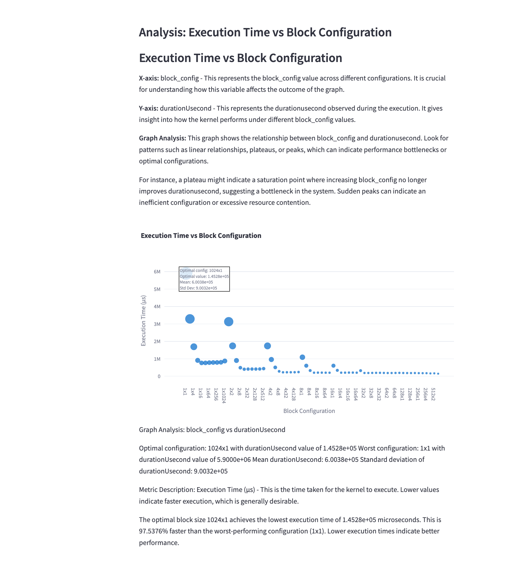
Mathematical Representation: \(T_{exec}(b) = f(b)\) where $b$ represents the block configuration and $f(b)$ is the execution time function.
Analysis: This graph illustrates how different block configurations affect the execution time of the convolution kernel. The goal is to minimize execution time. We observe that:
- Smaller block sizes (e.g., 16x16) often result in higher execution times due to underutilization of GPU resources.
- Larger block sizes (e.g., 32x32) generally reduce execution time but may plateau or increase beyond a certain point due to resource constraints.
- The optimal block size typically lies in the middle range, balancing resource utilization and scheduling overhead.
5.2 SM Efficiency vs Block Configuration
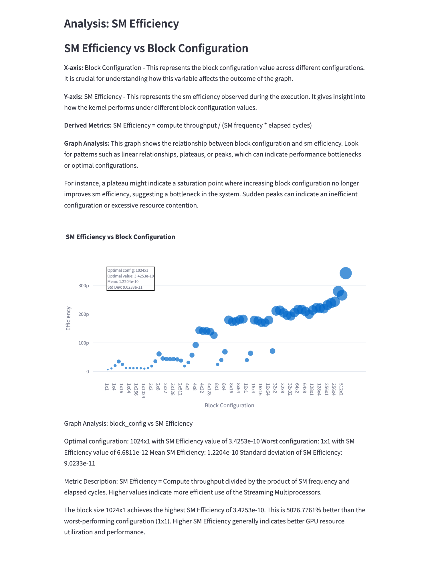
Mathematical Representation: \(E_{SM}(b) = \frac{\text{Active SM Cycles}(b)}{\text{Total SM Cycles}(b)}\)
Analysis: This graph shows how efficiently the Streaming Multiprocessors (SMs) are utilized for different block configurations. Key observations include:
- Smaller block sizes often lead to lower SM efficiency due to insufficient parallelism.
- Larger block sizes generally increase SM efficiency up to a point, after which it may decrease due to resource contention.
- The block size that maximizes SM efficiency may not always correspond to the lowest execution time, highlighting the need for a balanced approach to optimization.
5.3 Compute Throughput vs Execution Time
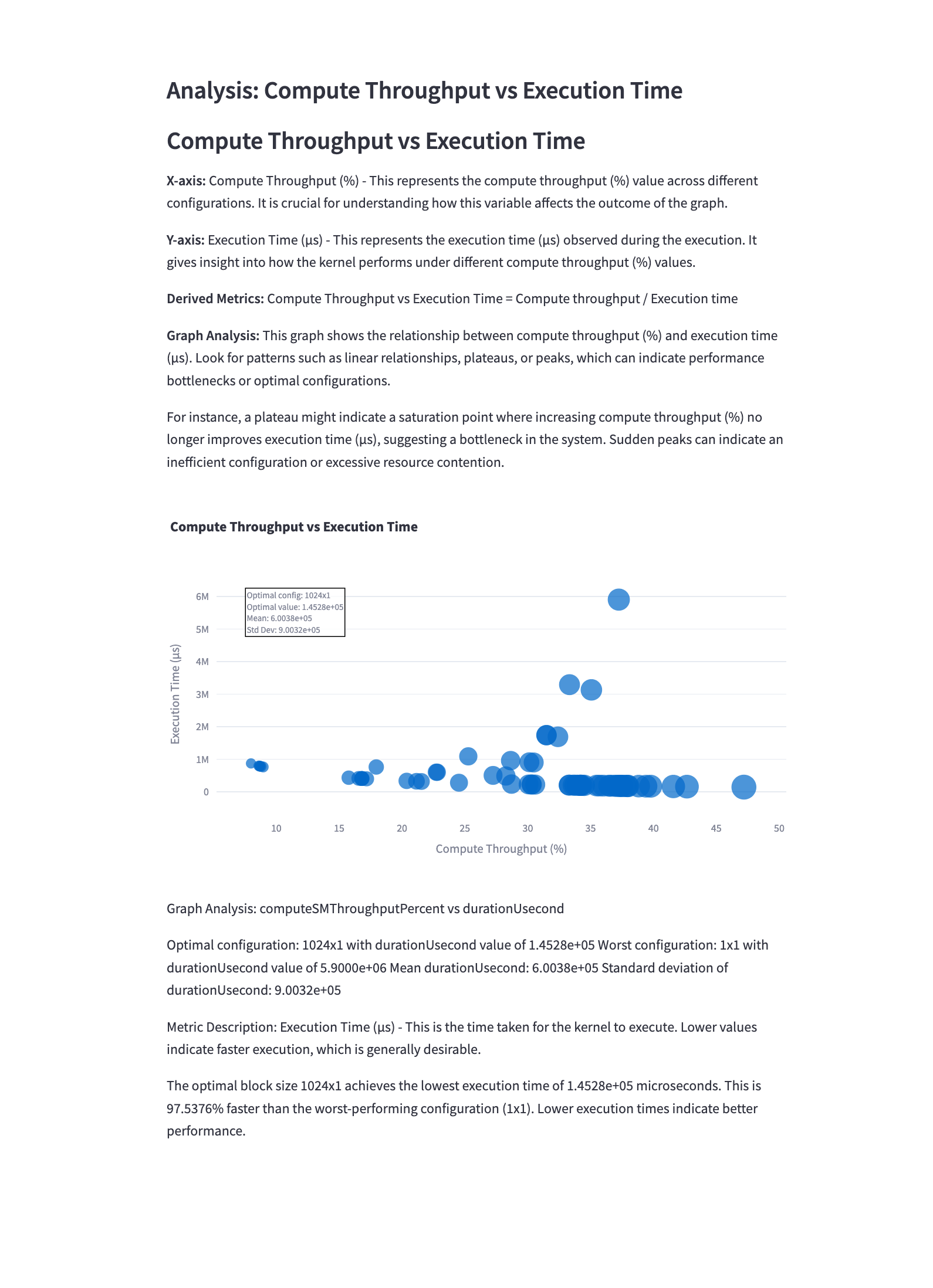
Mathematical Representation: \(\text{Compute Throughput} = \frac{\text{Total FLOPs}}{\text{Execution Time}}\)
Analysis: This graph illustrates the relationship between compute throughput and execution time. Observations include:
- There’s often a trade-off between high compute throughput and low execution time.
- Configurations that achieve high throughput with relatively low execution time are ideal.
- The graph can help identify compute-bound vs. memory-bound configurations.
5.4 Memory Throughput vs Execution Time
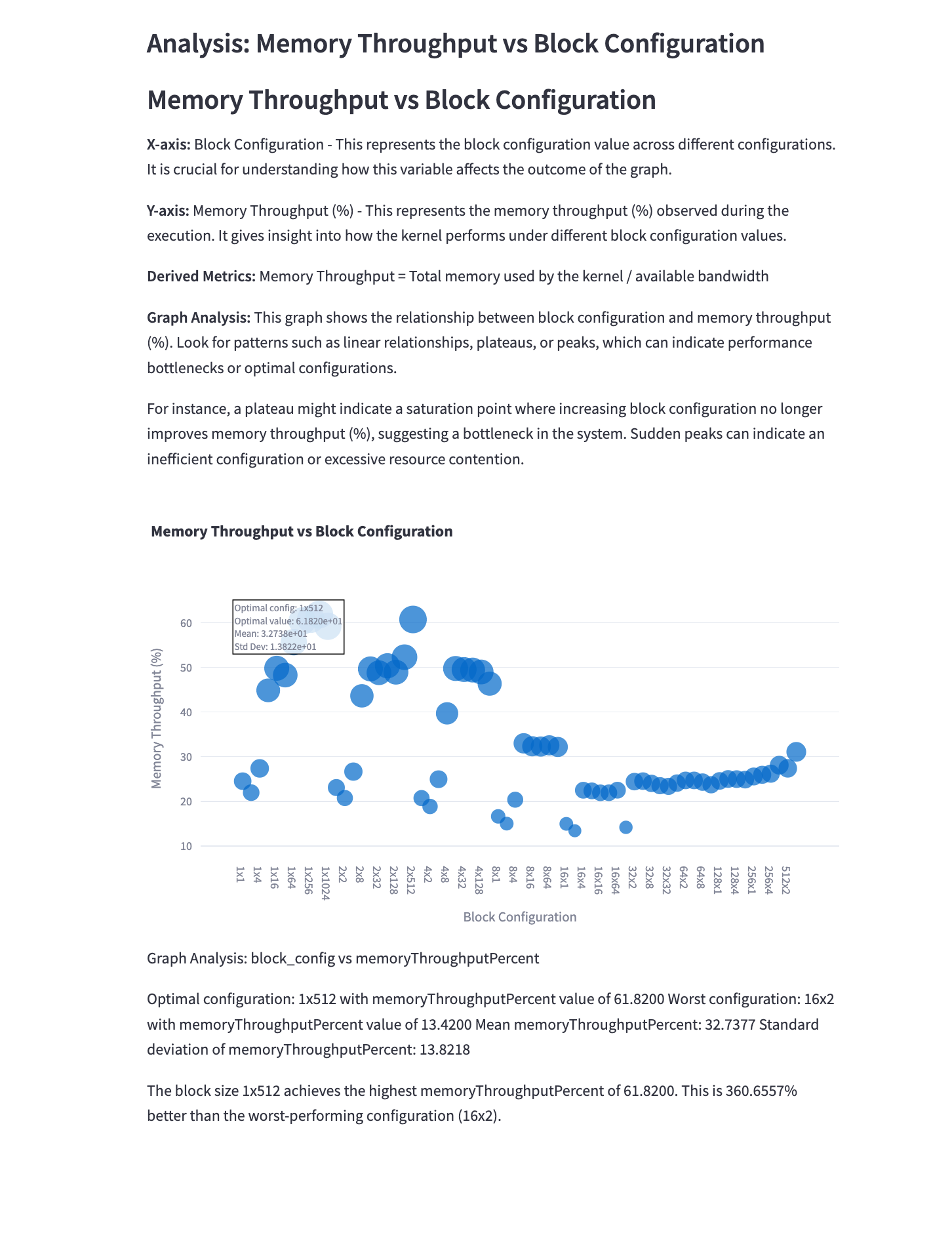
Mathematical Representation: \(\text{Memory Throughput} = \frac{\text{Total Bytes Transferred}}{\text{Execution Time}}\)
Analysis: This graph shows the relationship between memory throughput and execution time. Key points:
- Higher memory throughput is generally desirable, but not at the cost of significantly increased execution time.
- Configurations that achieve high memory throughput with low execution time indicate efficient memory access patterns.
- The graph can help identify memory bottlenecks in the convolution kernel.
5.5 DRAM vs SM Frequency Analysis

Mathematical Representation: \(\text{DRAM to SM Frequency Ratio} = \frac{\text{DRAM Frequency}}{\text{SM Frequency}}\)
Analysis: This graph compares DRAM throughput with SM frequency. Observations include:
- A balanced ratio indicates efficient utilization of both memory and compute resources.
- Imbalances can suggest either memory or compute bottlenecks in the convolution kernel.
- Optimal configurations maintain a balance between DRAM and SM utilization.
5.6 Cache Hit Rate Analysis
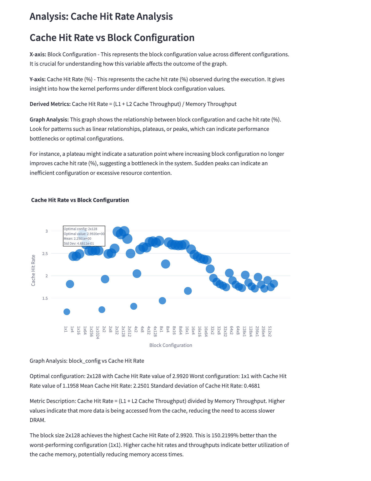
Mathematical Representation: \(\text{Cache Hit Rate} = \frac{\text{Cache Hits}}{\text{Total Memory Accesses}}\)
Analysis: This graph shows the cache hit rate for different configurations. Key points:
- Higher cache hit rates generally lead to better performance due to reduced DRAM accesses.
- The impact of cache hit rate on performance may vary depending on whether the kernel is compute-bound or memory-bound.
- Optimizing data layout and access patterns can significantly improve cache hit rates.
5.7 L1 Cache vs L2 Cache Throughput
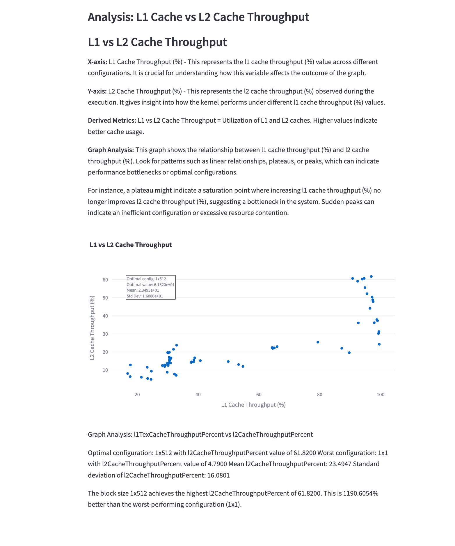
Mathematical Representation: \(\text{L1 Cache Throughput} = f(\text{L1 Cache Accesses})\) \(\text{L2 Cache Throughput} = g(\text{L2 Cache Accesses})\)
Analysis: This graph compares the throughput of L1 and L2 caches. Observations include:
- Higher throughput for both L1 and L2 caches generally indicates more efficient memory access patterns.
- The balance between L1 and L2 cache usage can impact overall performance.
- Optimizing for L1 cache usage can significantly reduce memory latency in convolution operations.
5.8 SM Utilization vs Memory Throughput
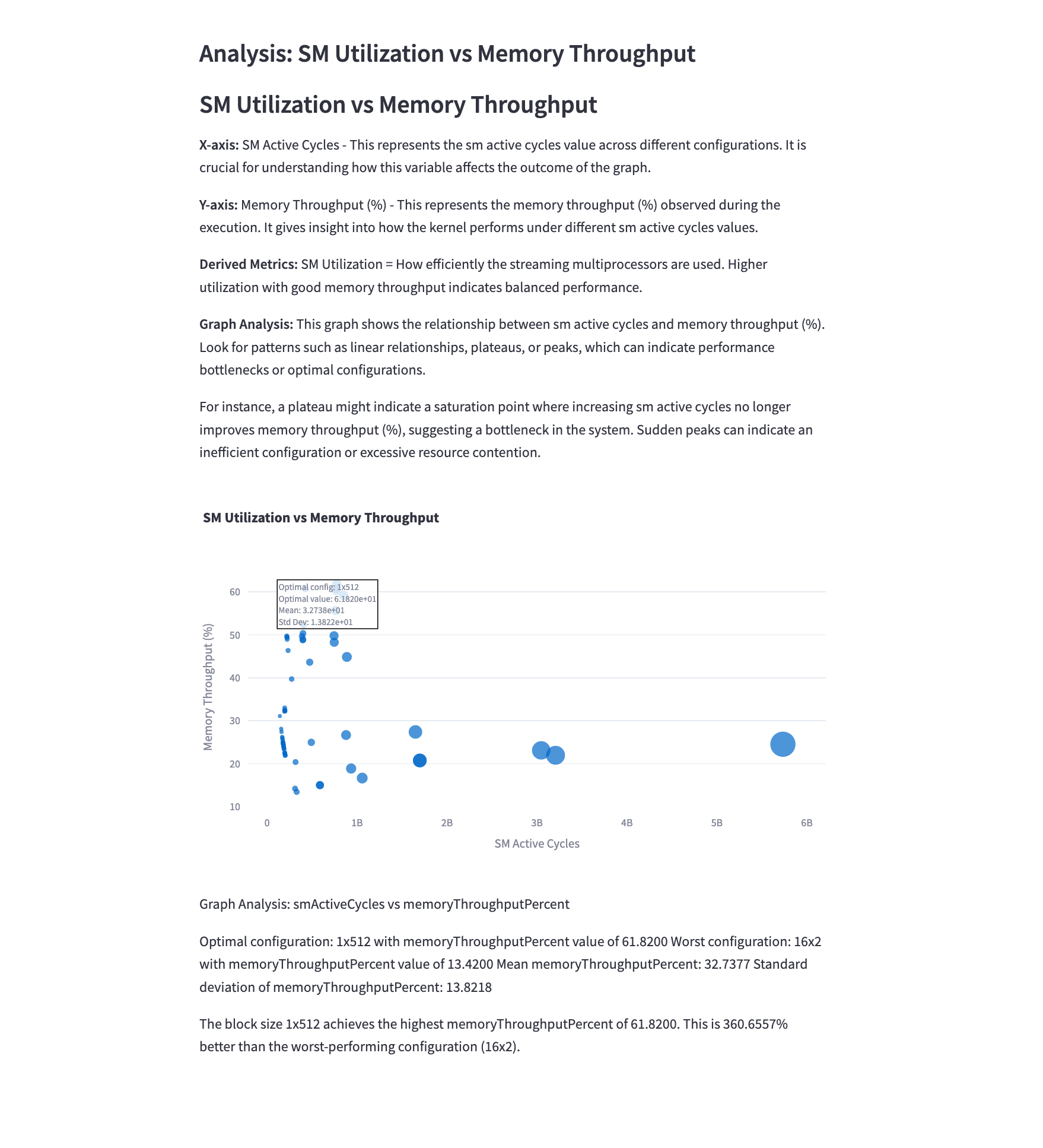
Mathematical Representation: \(\text{SM Utilization} = \frac{\text{Active SM Time}}{\text{Total Execution Time}}\)
Analysis: This graph illustrates the relationship between SM utilization and memory throughput. Key observations:
- Higher SM utilization with higher memory throughput indicates efficient use of both compute and memory resources.
- Configurations in the upper-right quadrant of the graph are generally optimal, balancing compute and memory efficiency.
- Points clustered along the diagonal suggest a well-balanced kernel, while off-diagonal points may indicate bottlenecks.
5.9 Achieved Warps vs Occupancy

Mathematical Representation: \(\text{Occupancy} = \frac{\text{Achieved Warps}}{\text{Maximum Possible Warps}}\)
Analysis: This graph shows the relationship between achieved warps and occupancy. Observations include:
- Higher occupancy generally correlates with more achieved warps, indicating better resource utilization.
- The relationship may not be perfectly linear due to other limiting factors (e.g., shared memory usage, register pressure).
- Configurations that maximize both metrics are typically desirable for optimal performance.
5.10 Performance Variability Analysis

Mathematical Representation: \(\text{Variability} = \frac{\text{Standard Deviation of Execution Time}}{\text{Mean Execution Time}}\)
Analysis: This graph illustrates the variability in execution time across different configurations. Key points:
- Lower variability is generally desirable for consistent performance.
- High variability may indicate sensitivity to factors like memory access patterns or thread divergence.
- Configurations with low variability and low execution time are ideal for stable, high-performance convolution operations.
5.11 Memory Bandwidth Utilization vs Block Configuration
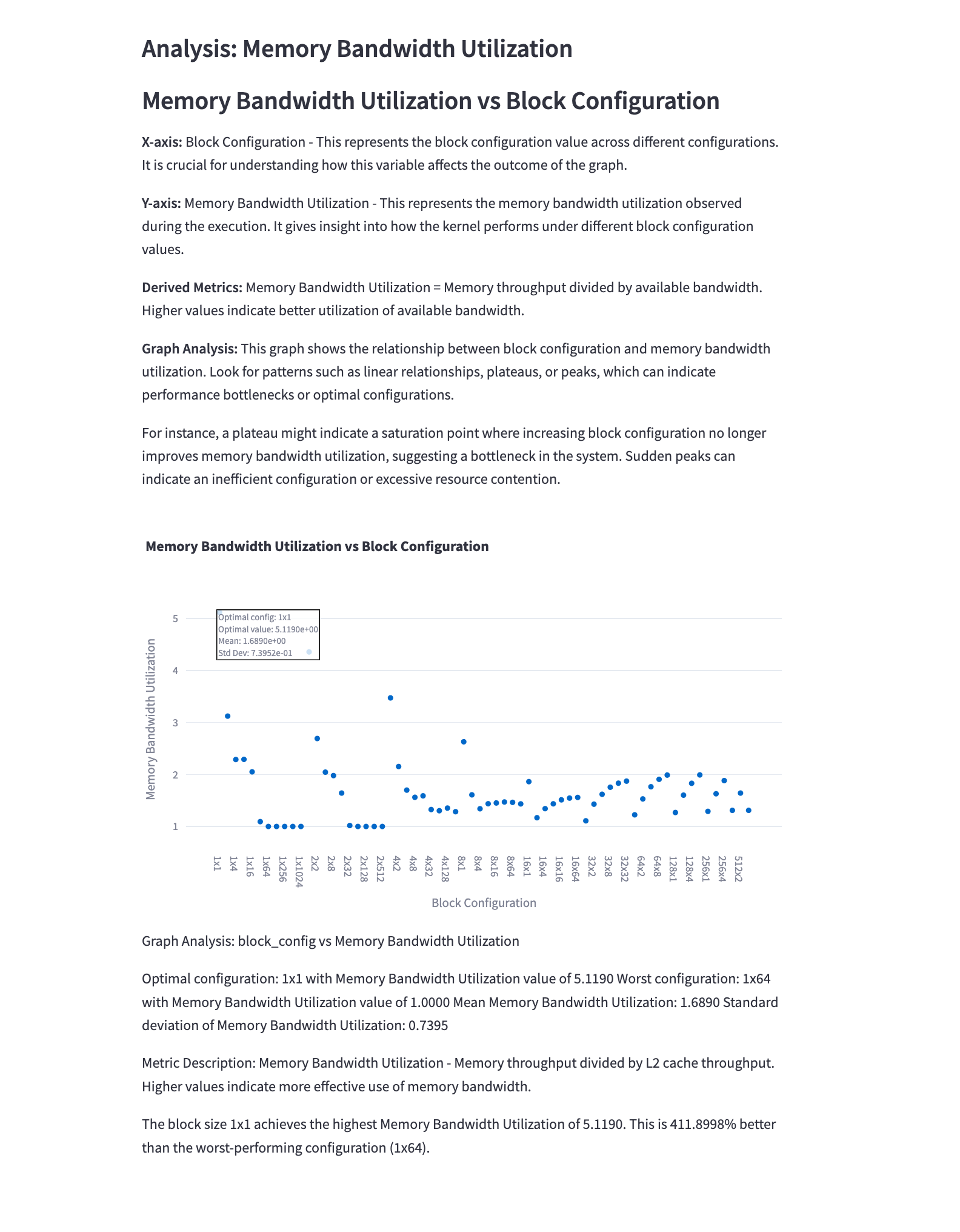
Mathematical Representation: \(\text{Memory Bandwidth Utilization} = \frac{\text{Actual Memory Throughput}}{\text{Peak Memory Bandwidth}}\)
Analysis: This graph shows how effectively the available memory bandwidth is utilized for different block configurations. Observations:
- Higher utilization indicates better use of available bandwidth, crucial for memory-bound kernels.
- There’s often a sweet spot in block size that maximizes bandwidth utilization.
- Configurations with high bandwidth utilization but poor overall performance may indicate other bottlenecks.
5.12 Register Pressure Analysis
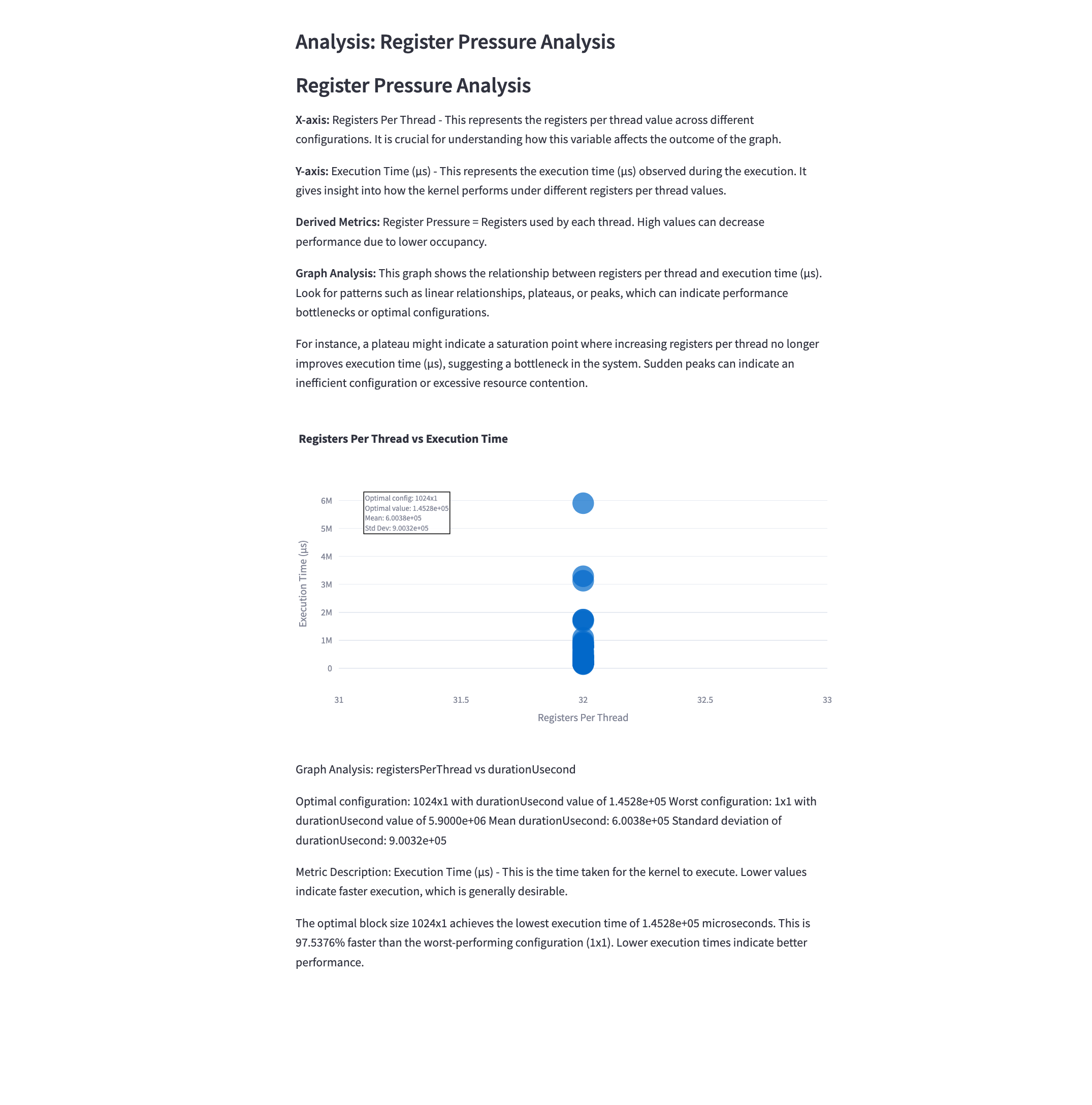
Mathematical Representation: \(\text{Register Pressure} = \frac{\text{Registers Used per Thread}}{\text{Maximum Available Registers per Thread}}\)
Analysis: This graph illustrates the impact of register usage on performance. Key points:
- Higher register usage can limit the number of concurrent threads, potentially reducing occupancy.
- There’s often a trade-off between register usage and performance; some increase in register usage can improve performance by reducing memory accesses.
- The optimal point balances the benefits of additional registers against the cost of reduced occupancy.
5.13 Elapsed Cycles Analysis
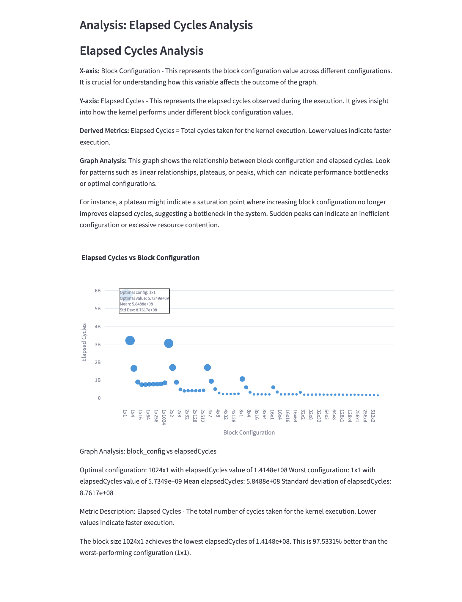
Mathematical Representation: \(\text{Elapsed Cycles} = \text{Clock Frequency} \times \text{Execution Time}\)
Analysis: This graph shows the total number of clock cycles elapsed during kernel execution for different configurations. Observations:
- Lower elapsed cycles generally indicate faster execution and better performance.
- The relationship between elapsed cycles and block configuration can reveal how effectively the GPU’s computational resources are being utilized.
- Configurations with low elapsed cycles but suboptimal performance may indicate other bottlenecks (e.g., memory bandwidth).
5.14 SM Active Cycles vs Duration

Mathematical Representation: \(\text{SM Efficiency} = \frac{\text{SM Active Cycles}}{\text{Total Cycles}}\)
Analysis: This graph compares the active cycles of SMs with the kernel execution duration. Key points:
- Points closer to the diagonal indicate higher SM efficiency, where most cycles are active cycles.
- Configurations with high active cycles but long durations may indicate memory or other bottlenecks.
- The ideal configuration maximizes active cycles while minimizing total duration.
5.15 Compute SM Throughput vs Block Size
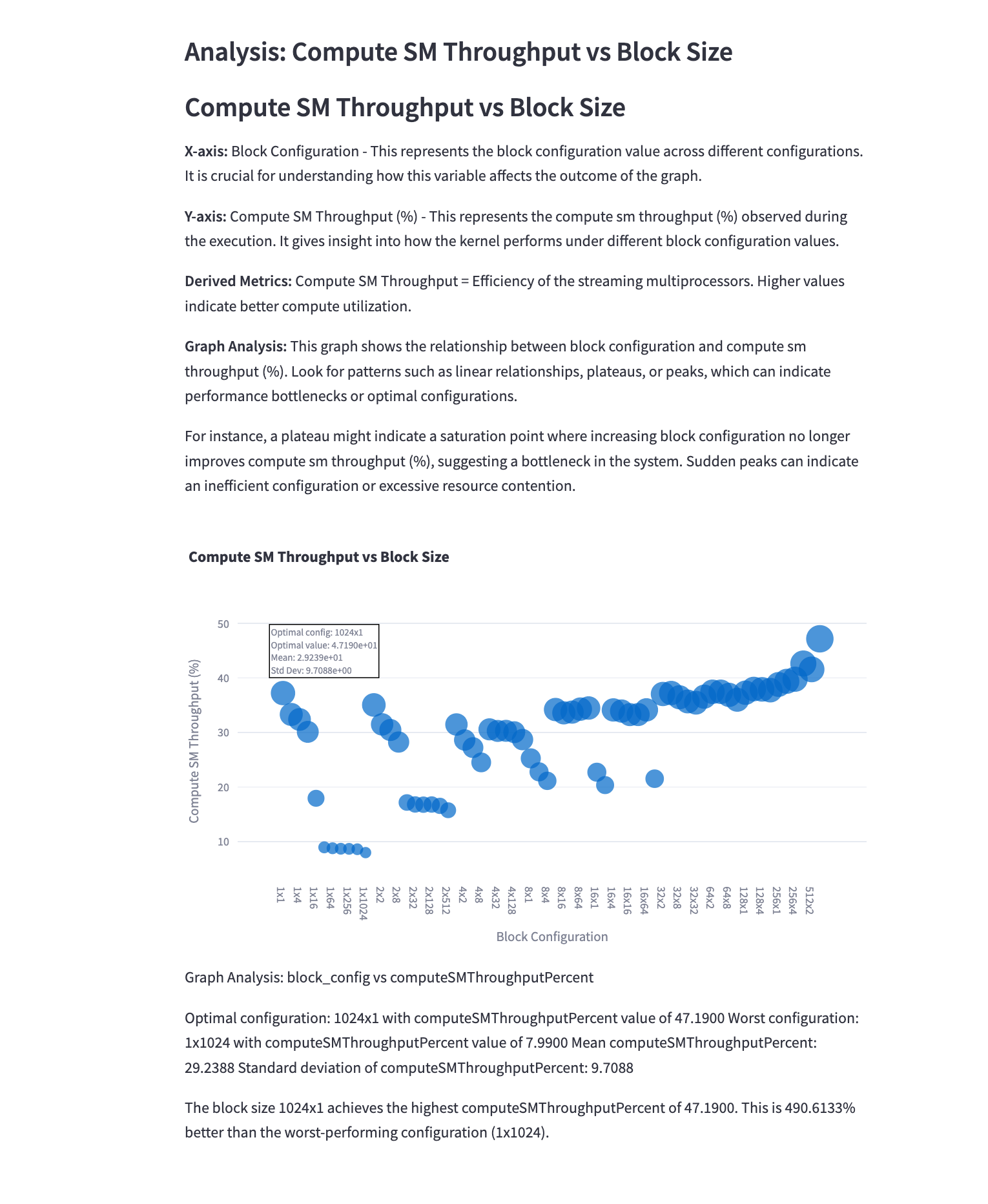
Mathematical Representation: \(\text{Compute SM Throughput} = \frac{\text{Instructions Executed}}{\text{Execution Time} \times \text{Number of SMs}}\)
Analysis: This graph shows the relationship between compute throughput of SMs and the block size. Observations:
- Larger block sizes often result in higher throughput due to better utilization of SM resources.
- There’s typically a point of diminishing returns, after which increasing block size doesn’t significantly improve throughput.
- The optimal block size balances high throughput with other factors like occupancy and memory efficiency.
These graphs provide a comprehensive view of the performance characteristics of 2D convolution operations on GPUs. By analyzing these metrics, developers can identify bottlenecks, optimize kernel configurations, and achieve better overall performance for convolution operations in deep learning and image processing applications.
6. Key Takeaways and Optimization Strategies
6.1 Summary of Key Insights
-
Block Configuration Impact: Block size significantly affects execution time, SM efficiency, and resource utilization. There’s often an optimal range that balances these factors.
-
Memory vs. Compute Balance: The relationship between memory throughput and compute throughput is crucial. Optimal performance often requires balancing these two aspects.
-
Cache Utilization: High cache hit rates, particularly for L1 cache, can significantly improve performance by reducing DRAM accesses.
-
Occupancy and Warp Execution: Higher occupancy generally correlates with better performance, but this relationship isn’t always linear due to other limiting factors.
-
Register Pressure: While using more registers can improve performance, excessive register usage can limit occupancy and overall performance.
-
SM Utilization: Maximizing SM active cycles while minimizing total execution time is key to efficient GPU utilization.
-
Memory Bandwidth: Effective utilization of memory bandwidth is crucial, especially for memory-bound convolution operations.
6.2 Optimization Strategies
Based on these insights, we can formulate several optimization strategies for GPU-based convolution operations:
1. Optimal Block Size Selection
Strategy: Experiment with different block sizes to find the optimal configuration.
Implementation:
dim3 blockSize(BLOCK_SIZE_X, BLOCK_SIZE_Y, 1);
dim3 gridSize((W_out + BLOCK_SIZE_X - 1) / BLOCK_SIZE_X,
              (H_out + BLOCK_SIZE_Y - 1) / BLOCK_SIZE_Y,
              C_out);
convolutionKernel<<<gridSize, blockSize>>>(input, filter, output);
Rationale: The optimal block size balances SM efficiency, memory access patterns, and occupancy. It’s often problem-specific and requires empirical tuning.
2. Tiling and Shared Memory Utilization
Strategy: Use shared memory to cache input data and filter weights.
Implementation:
__shared__ float tile[TILE_SIZE][TILE_SIZE];
// Load data into shared memory
// Perform convolution using shared memory
Rationale: Tiling reduces global memory accesses by reusing data loaded into shared memory, improving memory throughput and cache hit rates.
3. Memory Coalescing
Strategy: Ensure global memory accesses are coalesced for efficient memory transactions.
Implementation:
// Instead of:
float val = input[b][c][h][w];

// Use:
float val = input[(((b * C_in + c) * H_in + h) * W_in + w)];
Rationale: Coalesced memory accesses maximize memory bandwidth utilization, crucial for memory-bound convolution operations.
4. Loop Unrolling and Instruction-Level Optimization
Strategy: Unroll loops to increase instruction-level parallelism.
Implementation:
#pragma unroll
for (int i = 0; i < FILTER_SIZE; ++i) {
    // Convolution computation
}
Rationale: Loop unrolling can increase SM utilization and instruction throughput, potentially improving performance for compute-bound scenarios.
5. Register Pressure Management
Strategy: Carefully manage register usage to balance performance and occupancy.
Implementation:
__launch_bounds__(MAX_THREADS_PER_BLOCK, MIN_BLOCKS_PER_SM)
__global__ void convolutionKernel(...)
Rationale: Proper register management ensures high occupancy while providing enough registers for efficient computation.
6. Kernel Fusion
Strategy: Fuse multiple operations (e.g., convolution + activation) into a single kernel.
Implementation:
__global__ void convolutionActivationKernel(...)
{
    // Perform convolution
    // Immediately apply activation function
}
Rationale: Kernel fusion reduces memory bandwidth requirements and kernel launch overhead, potentially improving overall performance.
7. Mixed Precision Arithmetic
Strategy: Use lower precision (e.g., FP16) where accuracy allows.
Implementation:
#include <cuda_fp16.h>
__global__ void convolutionKernel(half* input, half* filter, half* output)
{
    // Convolution using half-precision arithmetic
}
Rationale: Lower precision arithmetic can increase computational throughput and reduce memory bandwidth requirements.
6.3 Performance Modeling and Autotuning
To systematically optimize convolution operations, consider implementing:
-
Analytical Performance Model: Develop a model that predicts performance based on kernel parameters and hardware characteristics.
-
Autotuning Framework: Create a system that automatically explores the parameter space (block size, tiling strategy, etc.) to find optimal configurations.
-
Profile-Guided Optimization: Use profiling data to guide optimizations, focusing efforts on the most impactful areas of the convolution kernel.
By applying these strategies and continuously analyzing performance metrics, developers can significantly improve the efficiency of GPU-based convolution operations, leading to faster and more efficient deep learning and image processing applications.